
混合精度演算の利用方法(Tensorコア)
本記事では、GPUSOROBANのインスタンスで混合精度演算を利用し、計算速度を向上する方法を紹介します。
GPUSOROBANは高性能なGPUインスタンスが低コストで使えるクラウドサービスです。
サービスについて詳しく知りたい方は、GPUSOROBANの公式サイトを御覧ください。
目次[非表示]
- 1.はじめに
- 2.混合精度を利用するための必要条件:
- 3.混合精度の仕組み
- 4.データセットのインポート
- 5.モデルの定義
- 6.モデルのトレーニング
- 7.改善結果
はじめに
この例では、多層ニューラルネットワークの一つであるCNN上で、画像を分類するためのトレーニング時間を短縮できることを示します。混合精度を使用することにより、FP16型で計算してもよいレイヤーとFP32型で計算してもよいレイヤーを自動的に識別し、画像の分類精度をほぼ落とすことなくトレーニング時間を短縮できます。今回GPUSOROBAN(A100, GPUメモリ:40GB)にて、混合精度の機能を利用してトレーニングを行った際、FP32型のみで計算したときに比べて約25%短縮することができました。参考記事1によると、Google Colab上のNVIDIA Tesla T4 GPUでは(同じモデルとバッチサイズを使用して)トレーニング時間を10エポックにわたって約33%短縮できる、という結果が得られています。
混合精度を利用するための必要条件:
ハードウェア側の条件:
・NVIDIA (Volta / Turing / Ampere) アーキテクチャ GPUのみ対応
・NVIDIA Driver release 418.xx+
・CUDA 10.1以上(*但し、NVIDIA Driver releaseに対応するもの)
・対応するcuDNNモジュールのインストール
・Tesla(Tesla V100, Tesla P4, Tesla P40 or Tesla P100)を利用される場合、NVIDIA driver release 384.111+ or 410を利用する必要があります。また、CUDA及びcuDNNについては、NVIDIA driverに対応するバーションを利用する必要があります。
ソフトウェア側の条件:
・TensorFlow version >=1.14.0-rc0
混合精度の仕組み
混合精度の仕組みはFP16型で計算してもよいレイヤーとFP32型で計算してもよいレイヤーを自動的に識別し、モデルのトレーニングを実施できることです。FP16型で計算したレイヤーにつき、アンダーフローが発生する場合、FP32型で計算するので、モデルの最適化精度を落とすことなく、トレーニング時間が短縮され、メモリ使用量が削減されます。
混合精度について、もっと知りたい場合、以下資料をお勧めします。
・Overview of Automatic Mixed Precision for Deep Learning
・NVIDIA Mixed Precision Training Documentation
・NVIDIA Deep Learning Performance Guide
・Information about NVIDIA Tensor Cores
・Post on TensorFlow blog explaining Automatic Mixed Precision
下記のセクションでは必要なライブラリーがインストールされているか、そして、Tensor Coreが入っているのかの確認です。
TensorFlow version is 2.4.1
Tensor Core GPU Present: True
データセットのインポート
CIFAR10 の画像データセットを tf.keras.datasets からインポートします。
画像の前処理として、画像の値をレンジ0 ~ 255からレンジ0 ~ 1に正規化します。
モデルの定義
画像の分類ができるように単純なCNNを返すための再利用可能なヘルパー関数を定義します。
Model: "sequential"
Layer (type) Output Shape Param #
================================================================================
conv2d (Conv2D) (None, 32, 32, 128) 3584
conv2d_1 (Conv2D) (None, 32, 32, 256) 295168
conv2d_2 (Conv2D) (None, 32, 32, 256) 590080
conv2d_3 (Conv2D) (None, 32, 32, 256) 590080
max_pooling2d (MaxPooling2D) (None, 16, 16, 256) 0
conv2d_4 (Conv2D) (None, 16, 16, 256) 590080
conv2d_5 (Conv2D) (None, 16, 16, 256) 590080
conv2d_6 (Conv2D) (None, 16, 16, 512) 1180160
conv2d_7 (Conv2D) (None, 16, 16, 512) 2359808
max_pooling2d_1 (MaxPooling2 (None, 8, 8, 512) 0
conv2d_8 (Conv2D) (None, 8, 8, 256) 1179904
conv2d_9 (Conv2D) (None, 8, 8, 256) 590080
conv2d_10 (Conv2D) (None, 8, 8, 256) 590080
conv2d_11 (Conv2D) (None, 8, 8, 128) 295040
max_pooling2d_2 (MaxPooling2 (None, 2, 2, 128) 0
flatten (Flatten) (None, 512) 0
batch_normalization (BatchNo (None, 512) 2048
dense (Dense) (None, 512) 262656
dense_1 (Dense) (None, 10) 5130
================================================================================Total params: 9,123,978
Trainable params: 9,122,954
Non-trainable params: 1,024
モデルのトレーニング
混合精度を用いない場合と用いる場合の比較を下記の関数(train_model)で、実施します。参考記事1では "optimizer = tensorflow.compat.v1.train.experimental.enable_mixed_precision_graph_rewrite(optimizer)" が使われております。TensorFlow2.4.0以降ではこのAPI自体がもはや実験的ではなくなるため、下記のコードに変更され、より高速にトレーニングすることができます。
optimizer = tf.compat.v1.mixed_precision.enable_mixed_precision_graph_rewrite(optimizer) *このような変更するだけ、時間短縮の度合いは34%から48%まで高まります。
*参考記事1のコードではscore = model.evaluate(x_test, y_test, verbose=0)という定義がなされていないバグがあり、参考記事2の通りで修正することで解消されます。
FP32型の場合の計算を下記の通り、行います。
Epoch 1/10
157/157 [==============================] - 25s 107ms/step - loss: 2.0124 - accuracy: 0.2686
Epoch 2/10
157/157 [==============================] - 15s 98ms/step - loss: 1.4031 - accuracy: 0.4937
Epoch 3/10
157/157 [==============================] - 16s 100ms/step - loss: 1.1473 - accuracy: 0.5937
Epoch 4/10
157/157 [==============================] - 16s 101ms/step - loss: 0.9442 - accuracy: 0.6699
Epoch 5/10
157/157 [==============================] - 16s 101ms/step - loss: 0.7919 - accuracy: 0.7237
Epoch 6/10
157/157 [==============================] - 16s 102ms/step - loss: 0.6781 - accuracy: 0.7650
Epoch 7/10
157/157 [==============================] - 16s 103ms/step - loss: 0.5930 - accuracy: 0.7942
Epoch 8/10
157/157 [==============================] - 16s 104ms/step - loss: 0.5058 - accuracy: 0.8261
Epoch 9/10
157/157 [==============================] - 17s 108ms/step - loss: 0.4280 - accuracy: 0.8560
Epoch 10/10
157/157 [==============================] - 18s 118ms/step - loss: 0.3564 - accuracy: 0.8801
59.6 % achieved in 175.5 seconds
下記のコードでは10秒間ほど、GPUを休憩させ、クールダウンさせます。
混合精度の場合の計算を下記の通り、行います。
WARNING:tensorflow:tf.keras.mixed_precision.experimental.LossScaleOptimizer is deprecated. Please use
tf.keras.mixed_precision.LossScaleOptimizer instead. For example
opt = tf.keras.mixed_precision.experimental.LossScaleOptimizer(opt)
Epoch 1/10
157/157 [==============================] - 23s 82ms/step - loss: 2.0110 - accuracy: 0.2667
Epoch 2/10
157/157 [==============================] - 11s 68ms/step - loss: 1.4662 - accuracy: 0.4639
Epoch 3/10
157/157 [==============================] - 11s 71ms/step - loss: 1.1991 - accuracy: 0.5745
Epoch 4/10
157/157 [==============================] - 11s 73ms/step - loss: 0.9855 - accuracy: 0.6501
Epoch 5/10
157/157 [==============================] - 12s 75ms/step - loss: 0.8191 - accuracy: 0.7134
Epoch 6/10
157/157 [==============================] - 12s 75ms/step - loss: 0.7092 - accuracy: 0.7517
Epoch 7/10
157/157 [==============================] - 12s 75ms/step - loss: 0.6126 - accuracy: 0.7858
Epoch 8/10
157/157 [==============================] - 12s 75ms/step - loss: 0.5219 - accuracy: 0.8203
Epoch 9/10
157/157 [==============================] - 12s 77ms/step - loss: 0.4464 - accuracy: 0.8487
Epoch 10/10
157/157 [==============================] - 12s 78ms/step - loss: 0.3835 - accuracy: 0.8714
62.5 % achieved in 130.5 seconds
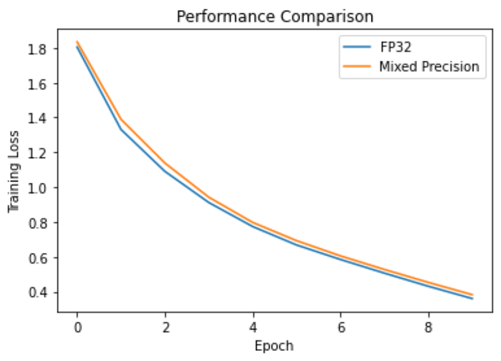
改善結果
トレーニング時間の短縮度合いを下記の通りに示します。
*optimizer = tf.compat.v1.mixed_precision.enable_mixed_precision_graph_rewrite(optimizer) *このような変更するだけ、時間短縮の度合いは34%から48%まで高まります。
Performance Improvement: 34 %
参考記事1:Mixed Precision Training of CNN
参考記事2:train_model(参考記事1のバグ修正)
参考記事3:Automatic Mixed Precision for Deep Learning
参考記事4:Automatic Mixed Precision (AMP) でニューラルネットワークのトレーニングを高速化
本環境には、GPUSOROBANのインスタンスを使用しました。
GPUSOROBANは高性能なGPUインスタンスが低コストで使えるクラウドサービスです。
サービスについて詳しく知りたい方は、GPUSOROBANの公式サイトを御覧ください。